In the late 2025 to the beginning of 2026 the usage of AI, especially the usage of Large Language Models (LLMs), became more and more prominent. With the two major contributions of OpenClaw and Claude Code agentic AI systems (so called AI assistents) become accessible to the public. Due to the lowered boundary of accessibility, on the social media now everyone talks about agentic AI systems, Claude Code and OpenClaw. Nearly every day there are posts about the latest feature updates, the must-have skill to install or just another vibe coded project. The development of agentic AI and coding assistants seems to be one of the most exciting developments in the recent decades. But have you ever asked yourself how well you understood the technology you are using? If yes, this blog post is for you! In this post I will try to provide an abstract, high-level and intuitive explanation how your initial prompt is passed down the model until the prediction of the next token. I will try to avoid deep mathematical theory and favor analogous examples. So this article is for everyone who wants to understand LLM on a intuitive level. At the same time this means that it is not a research post. Also, due to abstraction there will be statements not holding all the time true. This is the tradeoff, we have to accept.
Like a famous mathematician said once: Every Model is wrong. But at least some of them are helpful in understanding the world.
So I hope, this blog post will be helpful for at least some of the readers. If you really want to go deeper, after reading this article you will have the right buzzwords to go on.
The blog post is three part, where the parts build up on each other. In Part I, we will discuss basic LLM structure principles. We will start with a prompt, clarifying tokenization and embedding, and then explain the MLP transformer architecture and intuition, before arriving at the next predicted token at the unembedding stage. So the first part is entirely about arriving at prediction from given input. To this end, we assume an already trained model. Dealing only with inference time keeps this post more clean. May in a later post, we will discuss training phase separately.
We follow up by Part II, where agentic AI is discussed. Bulding up on the gained knowledge from the first part we will elaborate on situations where agentic AI may will fail. We will discuss the error accumulation problem in detail providing visibility and awareness with respect to the usage of fully autonomous systems. This section is not about telling AI bad, we will try to give a feel about robust agent engineering and design instead, and make the user aware of possibly pitfalls.
The final part, Part III, will likely be the most subjective one and reflect my argumentation on AI development. Bridging the fundamental concepts worked out in this blog post and the currently growing market needs, we will highlight the discrepancy between market demands, users requests and robust AI deployments, finishing with a personal opinion on that divergence. Thereby we will argue by three perspectives, the perspective of the field of cybersecurity, the users perspective, and the one of the growing AI market in general.
While walking through this entire post I will provide real-world examples, analogous, and pitfalls where thinks can go wrong including the root cause analysis, at any time possible.
There is a final Disclaimer I have to reveal. From my profession I am a cybersecurity specialist with strong background in mathematics. This said I am neither a AI researcher nor an AI company employee. All my reasoning will be based on fundamental mathematical concepts I learned during my studies in theoretical mathematics, enriched by day-to-day experience in the field of cybersecurity. To make this post accessible to a public audience things need to be simplified or just explained in a way that is easy to understand for humans but ineffective to implement. So, none of the insights presented here should be implemented one by one into production. There is always space for fine-tuning and improvement. Nevertheless, I guarantee you, that after understanding this post you will likely know a lot more about LLMs than the average user.
Part I: Discussing the LLM Pipeline
The Prompt
Everything starts with natural language. In essence a prompt is just a bunch of words that the LLM will process. There is an entire field researching on prompt engineering. I.e., finding a good formulated prompt for specific given task. However understanding the aspects making a prompt good or bad requires deeper knowledge of the following stages in the models pipeline. So for the moment imagine and accept that you are allowed to enter any text you like.
Nevertheless, it already makes sense to think about safety and security aspects at this stage here. Even without understanding anything about AI, we will likely agree on the following concern:
- The system prompt should never be made out of untrusted input. Untrusted means here either user input; or in agentic loop systems the results from previous iterations of the agent. While this observation sounds obvious, we will later see and understand that this first assumption is already broken in many public used AI applications. E.g., the Microsoft Copilot 365 “EchoLeak” Vulnerability and the Gemini Calendar Invite issue
As we can see, thinks can go terribly wrong if untrusted input is processed by the LLM! Anyways, attacking AI systems is out of the scope of this post. If you are interested in such topics, familiarize yourself with the basics of (indirect) prompt injection, jail breaking, targeted label attacks and adversarial machine learning in general.
Tokenization
The prompt is basically a string, but neural networks operate on numbers. So the very first step is the conversation of the prompt to a numerical representation. If you think about that problem for a moment, you will likely come up with a major constraint in this step Every text input have to be able to be converted into numerical representation. This fundamental insight makes clear, that we could not simply attach each text in this world a number. The reason is, that we can construct infinite about of strings, but just have finite numbers of values representable by modern computers. The intuitive solution to that problem is to split up the text into words. Now in theory we only need to handle a mapping from words to numbers. I.e., we need only as many numbers as possible words, and texts become sequences of numbers. But think twice, what happens to an input like Helllo (simple typo). This is a complete new word for that approach, and may not have any numerical representation yet. Anyway, the intuition is right, we just need to split things a bit more. Let us define that the set of tokens are the letters from A-Z, a-z, and 0-9. Now, we can represent every “normal” text as a sequence of numbers. E.g., “Hello” becomes [8, 5. 12, 12, 15] assuming a simple one-to-one mapping between alphabet positional index and integers. While this may sound suitable it still does have two issues:
- We did not have mapped special cases like
ä,ü,%, and very important emojis - The word is now split so much, that we can not any more tell the difference between a
borigination frombenignorbad
The solution to both of these problems is called Byte-Pair-Encoding. This algorithm is the one used in the majority of tokenizers applied in modern LLM architecture. In the next subsection we will formalize its mechanics.
Byte-Pair-Encoding
The algorithm starts with a set of all values representable in a byte. I.e., 256 possible values. Remember, from computer science perspective everything is just a sequence of bytes. Starting with this initial set it learns a vocabulary of a pre-defined size \(\lvert V \rvert\) by processing “training” texts. A common value for the parameter is about \(50k\). The steps are as follows:
- Initialize by setting \(V\) to all symbols (in the following denoted as tokens) representable by one byte
- Build an intermediate set \(M = V \times V\). I.e., all possible combinations of the tokens already present in \(V\)
- Calculate the frequency of occurrence for each token in \(M\) over the given set of training texts
- Take the one token out of \(M\) with the highest frequency and add it to \(V\); Then continue with step (2) until the pre-defined size of \(V\) is reached
Before diving deeper, let us summarize the algorithm by a small depiction including an example.
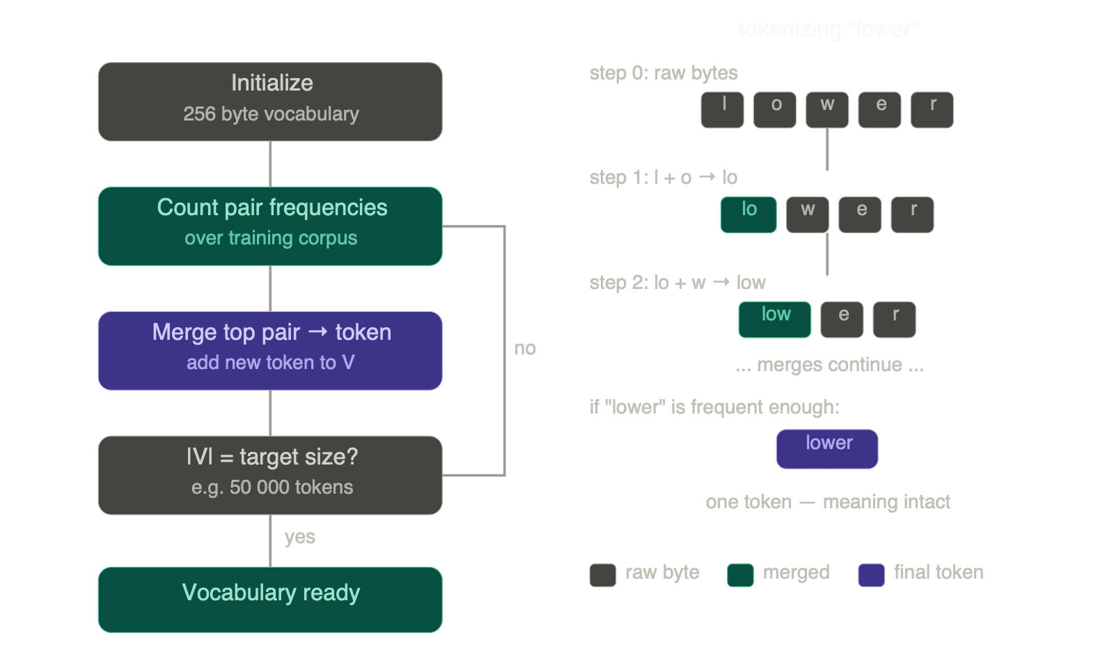
Notice, the following three key properties of Byte-Pair-Encoding
- Every input string can be represented as sequence of numbers. In the worst case by splitting up into the individual bytes
- High frequency words like
an,the, etc. will be encoded into one token keeping the semantic structure. - Since at each step the next highest possible combination is added, the Token set becomes an ordered set decreasing by means of frequency of occurrence in the training data.
For the number presentation, we now can just use the index in the list V. E.g., the is on 311 position in V, so the mapping becomes TOK(the) = 311.
Perfect, we have numbers! Now let us talk about the thinks could go wrong!
When Tokenization “surprises” us
Even without knowing anything about AI and LLMs until here, we can make some deliberate observations. Did you ever ask yourself what happens to your prompt if it contains domain specific language never seen during tokenization; Or even worse encrypted / obfuscated byte garbage resulted by pasting a strings output to the LLM and ask about triage in the scenario of malware analysis?
If yes, feel free to skip this part. If not here is the honest truth.
Ok, let us consider the word understand, since we want to understand something for today. Imagine a scenario, where the tokenization layer learned the tokens under and stand but not the combined word. (Remark: This example is demonstration purpose only. Current tokenization will commonly handle the word as one token!). In that case your human input is understand, a keyword related to educational content, but the LLM will see under, a directional instruction; and stand, another positional phrase. So just by tokenization the meaning of your intended input entirely shifted from education to positional arguing.
This is a real world problem, especially, when using a general purpose model on domain specific tasks!
Another issue is the high entropy input. Taking, e.g., the garbage string .bakcruciallilli from the .text section of a binary. A human may clearly indicate this as obfuscated indicator, however the LLM may see [.bak, crucial, lilli] and starts reasoing about backing up crucial files of the user Lilli. Beside this we likely see a lot of single byte tokens in the input stream, just because the input word is not from human language. These single byte tokens have usually low frequency in the training set, yielding that the model was not fully trained on these tokens. More on that later. For the moment it is enough to get the intuition that this may yield bad prediction results.
Wrapping up Tokenization
To wrap up, we can already formulate two major insights about a good prompt:
- Good prompts are low entropy ones
- If the model was not trained on your domain specific task accept the risks of failure
The entropy issue is by the way the reason why LLMs constantly fail on automated malware tasks. There are ways to improve this, by using so-called Entropy firewalls and input structure markers, however this is out of the scope of this blog post. For today consider malware the natural enemy of LLMs. In general, it is worth to mention that the requirements of cybersecurity and the strength of LLMs is still orthogonal in the current state of development.
From Tokens to Embeddings
Since we not have sequences of numbers one may think that we can directly feed them to the actual model, however there is a major issue we will discuss in this section. Our number sequences do not pose any metric formalizing semantic distance. E.g, take the two words dog and cat. They may have the tokens 123 and 456. But what does these numbers mean to the model? Are they close (related) to each other, or not? The answer is that the model is not able to tell this yet. The main task of an embedding is to provide a mapping, taking a token and assign it an embedding vector. In the space of embeddings there is a metric (measure of distance) capturing how related the embedding vectors are.
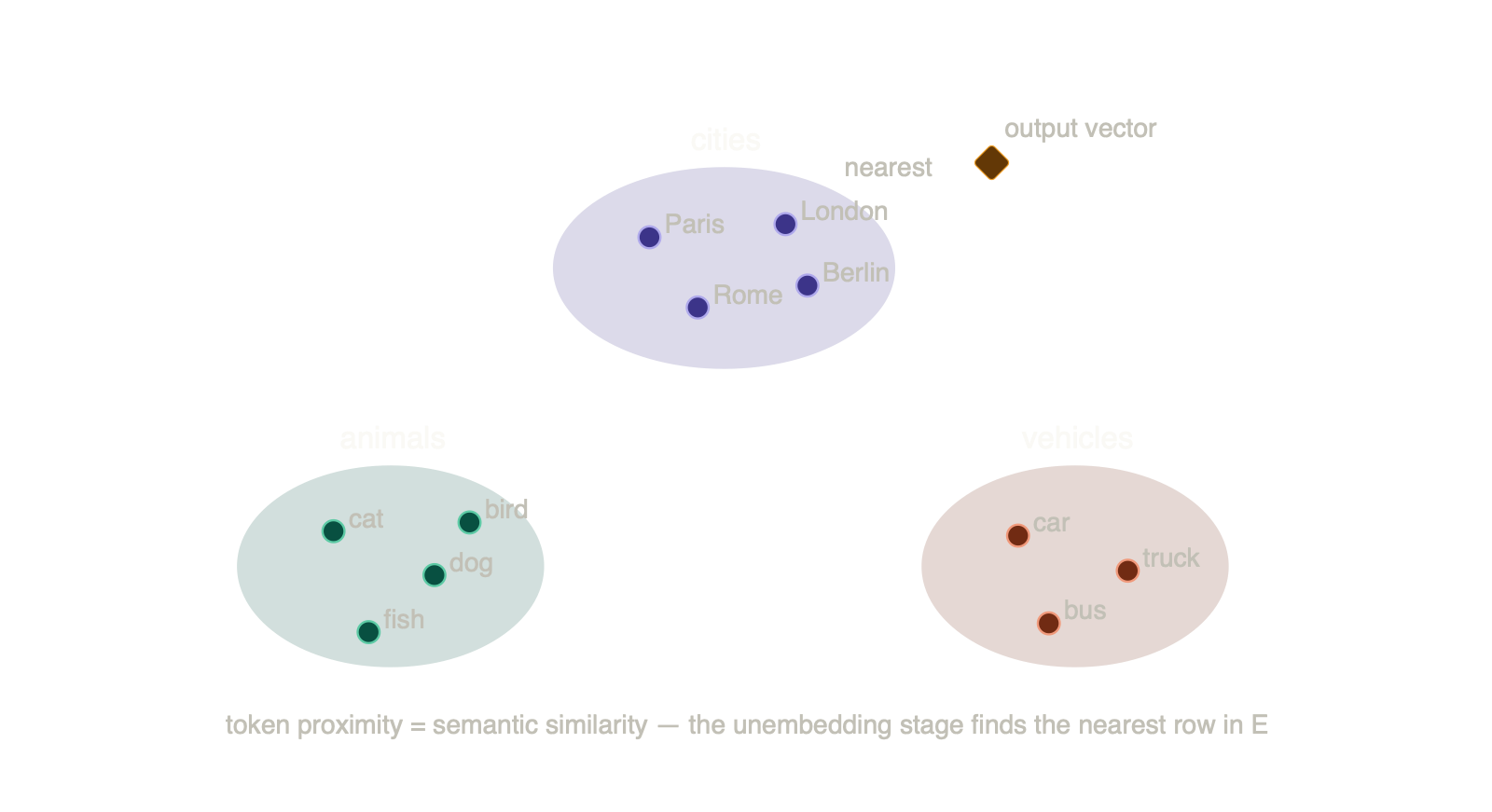
The embedding \(E\) does allow us to map every possible token to a vector in the embedding space. This is usually done by defining the embedding as a matrix \(E\), where the \(i\)-th row corresponds to the embedding vector of the \(i\)-th token in the vocabulary. This allows fast lookup. If we want to retrieve the embedding of a specific token, we just need to look up the row. But wait, by this definition it means that we need to know the embedding mapping already when defining it. The classical chicken-and-egg situation. To resolve this situation modern approaches work as follows. Initially, we guess the correct embedding, then we check if they are “good”. Since we do not know anything about the correct embedding initially, our guess does not matter and we can initialize the embedding Matrix \(E\) rows completely random. This is exactly how nearly every modern LLM works. Start with a random embedding matrix and update the values during training. So the embedding is never defined explicitly, it is learned implicitly during training. This is the reason it is called end-to-end learning.
From here on you may have some intuition on how to arrive at an embedding vector from a given token. Let us explore the “inverse” operation from an embedded vector back to a token. In the so called unembbeding stage the given embedded vector will be parsed back to their token representation. There is a fundamental and easy insight. These two operations must somehow be inverses of each other! If you listened to your algebra teacher well, you immediately spot an issue here, the embedding matrix \(E\) is not invertible by any means (typically not even quadratic matrix). So how can we get back to the tokens space.
Let us explore this by example. We are looking at the embedding Matrix \(E\) again. For each row of that matrix it is easy to get the corresponding definition due to the nature of the embedding itself. Remember the \(i\)-th row was the \(i\)-th token. So whenever we are questioned to convert an embedded vector back to token, which is contained in the embedding Matrix \(E\), the task becomes trivial. Just look up the index and return it. If we are confronted with a vector being not a row of \(E\), our next best option is to take that rows, which is “closest” to that vector. So what we can do with our given vector is to calculate “closeness” of it to each of the rows of \(E\). The one row which poses the most equality is the one we take. Since there is always the closest candidate, even if all are miles away, this approach ensures, that we always can go back from embedding to token layer.
In mathematical notion, one may calculate the scalar product (dot product) between the vector and all rows of the embedding matrix. If the dot product is zero, this means geometrically, that the two vectors are orthogonal. So entirely no relation between them. If the value is not null, there is some relation. Still, to distinguish between more or less “closeness”, we need some kind of normalization. Think of the following, vectors may being nearly orthogonal by means of direction can still contribute in high dot product if one of the vectors does pose a large length. Let us demonstrate this issue with the following two vectors in two-dimensional space.
\[\begin{align} x &= (0.1, 1), \\\\ y &= (1000, 0), \\\\ dot(x,y) &= 0.1 \cdot 1000 + 1 \cdot 0 = 100 \end{align}\]The vectors \(x\), and \(y\) are nearly orthogonal. I.e., in the language of the embedding space they are semantically far away. Still the dot product is very high, just because the vector \(y\) poses a high length. Normalization solves this problem. After dividing each vector by its norm, it will have length one and equally contribute in the dot product. Thus, only directionally relations were captured. This is the one sentences you need to keep in your mind, semantics relationship is measured in the embedding vector space by means of directions (angular distances)!
To this end, normalization is required. Phrased in other words, without proper normalization long vectors will contribute to semantic similarity without actually looking at the semantic direction.
The normalized dot product
\[similarity(X, Y) := dot(X,Y) / (\lvert X \rvert \cdot \lvert Y \rvert)\]is also denoted as cosine similarity in the domain specific language. Also, due to the normalization all “distances” are between \(-1\) and \(1\), where \(0\) means no relation, \(1\) means identical direction and \(-1\) opposite directions. Again, remember, when we talk about semantic distance, we will actually refer to angular distances! Keeping the values bounded also contributes to numerical stability.
This approach does pose another advantage. We do not need to learn and store a specific unembedding matrix. If you write down all these operations on paper, you will observe that calculating all these dot products is equal to a multiplication with the transposed of the embedding matrix. This phenomenon is called weight tying and saves a lot of bytes, since we only need to store once.
A mindful reader now may questions about the quality of the token we obtain, in case that our initial embedded vector is just not align with any row from the embedding matrix \(E\). The honest answer, the quality can be very bad and is a crucial issue in LLMs. Each token generated under certain input is just a conditional probability of being that this is the right token under the constraint of the previous input. We will hopefully understand later more about this.
If your intuition is good, you now may end up with the following question: What happens to the rows corresponding to low-frequency tokens in the training data. The answer is simple but fundamental. If a token has low-frequency in the training data, the corresponding row in the embedding matrix will stay nearly random. Hence, we have a random embedding vector. The issue with randomness is it can be “semantically near” to any other vector in the vector space just by geometric accident. Imagine the following situation, you have low-frequency token \(z\), yielding a nearly random embedding vector \(z_{e}\). By accident this vector is close to the embedding vector of the word dog. Now the following up pipeline will always think you want to reason about dogs, however actually, the \(z\) may was raised by “bad tokenization”. This is remarkable since during tokenization we already noted that low-frequency tokens and high entropy prompts are bad. Now we found another reason for the sake of that one layer deeper in the LLMs architecture.
If you wonder how to know whether your input contains low-frequency tokens or not, then the answer is that you can not know for sure. However, there are two possible heuristics you can check. Both require that you are able to tokenize your input on your end.
- Checking the vocabulary coverage: Assume you have an input prompt of \(k\) words. After tokenization, you obtain \(N\) tokens. Set the coverage ratio \(R\) to \(R = N/k\). If \(R\) is close to one nearly all words from your input prompt are contained in the set of vocabulary. I.e., the model learned on these words during training phase, increasing the chance for stable and well learned inference. So you can stop read here. On the other side, if \(R\) is large, this may indicate bad coverage or not. A typical prompt does pose \(R \approx 2.0\) or below, however natural language does have a lot compound words like unimportant. Here splitting into un and important is actually desired. For the sake of the latter, high \(R\) does not necessary mean low-frequency tokens in any case.
- Exploiting the Token positions: If you recall how Byte-Pair Encoding is learned, at each step the most frequent adjacent token pairs are merged and added to the vocabulary. This yields an interesting property: tokens with numerically higher indices were added later in the process, meaning they represent combinations of tokens that were not frequent enough to be merged earlier. I.e., they were less present in the training data set. If they had been frequent enough, they would already have been merged in a previous step. As a consequence, the encoded vocabulary forms an approximate frequency ranking by index. Lower indices correspond to higher-frequency tokens, while higher indices to lower-frequency ones. We can exploit this as a lightweight heuristic. Without access to the original training data, we can estimate which tokens in an input prompt are likely low-frequency. Given vocabulary size \(\lvert V \rvert\) (typically public knowledge for major models), we define a threshold \(T = 0.8 \cdot \lvert V \rvert\). Any token \(t_i\) with \(t_i >> T\) is likely a low-frequency token relative to the rest of the vocabulary. Counting or flagging these tokens gives a rough quality signal for the input prompt.
This heuristic has two fundamental weaknesses worth being explicit about. First, we are measuring relative frequency within the training data, not absolute frequency! A token just above the threshold might have appeared millions of times during training, it simply appeared less often than the tokens below the threshold. We have no visibility into the actual frequency distribution, only the rank ordering! Second, the distribution within the high-index region is completely unknown to us. The upper \(20\%\) of the vocabulary by index could contain hundreds of tokens each seen only a handful of times, or it could contain tokens seen millions of times that were simply merged late due to the specific order of byte-pair encoding iterations. The threshold is a statistical approximation, not a hard boundary between well-trained and poorly-trained embeddings! Despite these limitations, the heuristic is useful in practice precisely because it requires no access to training data. Only the vocabulary size, which is publicly documented for all major models is required.
I guess this is the right point to tell you about the so-called hyperparameter \(d\), which reflects the models size. I already told you that each row of the embedding matrix \(E\) will be reflecting on token. Hence, the row count of that matrix is equal to the vocabulary size \(\lvert V \rvert\) (Each token becomes one row!). However, how long should each of these rows be? This answer is defined by the parameter \(d\) and is up to so-called hyperparameter tuning. One of the modern LLMs secrets. Anyway, I will try to give some intuition on what happens with to small and to large parameter values. Since I promised to not drift up into mathematical reasoning let me give you a real world analogy. Remember, that semantic relationship is encoded by “directions” in the embedding space. Considering a two-dimensional space, and someone questions you to place the maximal possible fully independent directions into that space. Your natural solution will be to take the two axis, x-axis and y-axis. Only these two directions have nothing in relation with each other. Every additional “direction” you want to add will become a combination of that two axis. If the same riddle is asked for three-dimensional space you will come up with a solution providing three axes. So in generally increasing to a \(d\) dimensional space you will be able to store \(d\) fully semantically independent directions. Wrapped in other words, if \(d\) is to small there are just now enough directions you can safely distinguish from each other! But remember distinguishing directions means distinguishing tokens, which were deduced from words. So the value of \(d\) becomes an indicator of how much information can be encoded before collapse. If this was still too mathematical for you, imagine a small room (small \(d\)), and you want to fit \(1000\) people into. All people will be very close to each other making it hard to tell which ones are close when looking into the room. For a taken person, many others will be close! We have simply not enough capacity to store all these persons in that room. Even worse, if a new on is joining the room, this person will be close to someone may be not related to just by geometric accident. For our LLM this means, small \(d\) will not allow differentiating well between different meanings from the input data. On the other side a ridiculous large \(d\) will require a lot of computational resources and cause something called curse of dimensionality. One can mathematically show that if the dimension is just high enough, all vectors will be of equal directional distance. So also in that case we lose semantic comparability. The embedding becomes useless!
That’s it! We have discussed the embedding and elaborated on how to invert it. We have accepted that the embedding matrix values are randomly initialized and updated by some learning magic not discussed here. At this step nothing is learned from knowledge point of view. We have just discussed encoding and decoding. If different vocabulary sizes are used on the in- and output side we discussed encoders by accident. Even if these steps are not related to the LLM directly, we observed how it could impact our results when working with LLMs.
The positional problem
For the entire sake of this post we just discussed on a single token, so ordering was not relevant. However, common user input composes multiple tokens, where ordering is essential. E.g.,
The cat bite the dog.
The dog bite the cat.
Without relevance of ordering, both inputs will have the same representation in embedding space. There exists multiple approaches to establish an ordering. However, the positional encoding is out of the scope for this blog post. So for the moment think of it as a simple addition of positional information:
\[{input}_i = {token\_embedding}_i + {positional\_encoding}_i\]If you want to learn more about that topic, you can research on Sinusoidal position encoding and Learned positional embeddings. The latter is the approach used in modern LLMs.
Learning the Knowledge (Attention / MLP)
If you followed this blog until here, your initially entered prompt is now tokenized and embedded into a vector space with semantic (distance) meaning and enriched by positional information. So you have a sequence of enriched embedding vectors \(x_1\), … \(x_N\), where \(N\) is the amount of tokens used to represent your input prompt. Usually, we write this data in form of the state matrix \(X = (x_1, ..., x_N)\), where each column correspond to one token embedding vector. It may worse to mention, that all these steps are highly independent and well easy to execute in parallel.
Now it gets actually time to ask, where does the LLMs knowledge come from? This question is actually twofold! Knowledge always corresponds to factual data and contextual information. Consider the following example, where someone requests you to tell everything you know about a bank. So what is your answer? It depends on the context! Is the discussion about finance or the bank to sit on. The LLM will take the context from the surrounding words (i.e., tokens) in your input prompt.
On a high level view, if the LLM is operating on the following prompt
[PROMPT]
I need some money, where is the next bank?
It will apply the following steps:
- Use multi-head attention to establish context between each of the words. I.e., how much does each token attend to the other one. In the above prompt the model may observe the relation between money and bank, pushing the bank more into the direction of finance
- Once context is enriched, knowledge needs to be looked up for each token. E.g., bank was previously enriched by finance, now the MLP block will look up the corresponding knowledge of “bank + finance”
This is quite the same way humans operate. We first establish context, then retrieve out learned knowledge!
In the language of the model the first step is achieved by multi-head attention, the second by so called MLP Blocks. The belief by current state-of-the-art research is, that the learned knowledge is stored in the weights of the MLP Blocks. Typically, a modern LLM does have several of these layers (attention + MLP) chained after each other.
Before exactly understanding how attention and MLP works, let us illustrate the high-level view.
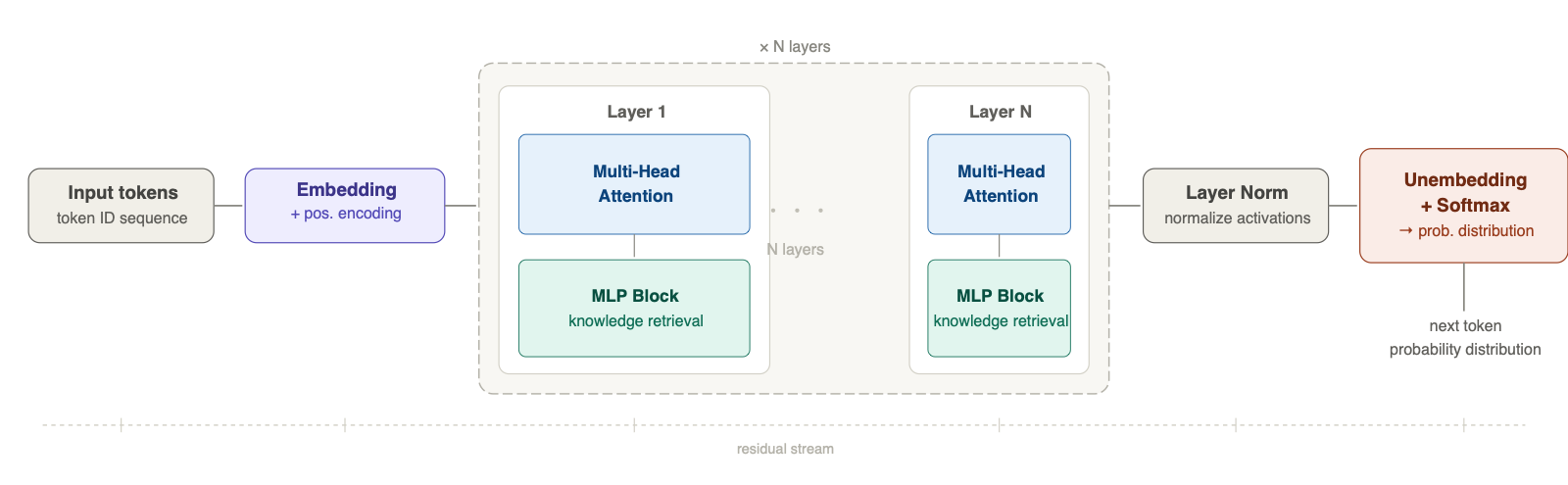
Since it is so fundamental, let us repeat it again! The MLP layer are twofold. They pose a so called multi-head attention, and the actual MLP block.
- The attention tries to answer the question of contribution of each token to is previous and followers. So for each token there are calculated values that keep track of how much these tokens contributes to others and how much other tokens contribute to itself. This is important to establish contextual relation over the prompt
- The MLP Blocks are basically a chain of two linear mappings cut by a non-linear activation function, which are believed to hold the actual knowledge by a key-value store mechanism. More later on this.
Minor Words about the Multi-Head Attention
So far our token has been embedded into a vector and enriched with positional information. But there is still a fundamental problem. Each token has been processed entirely in isolation. The embedding of the word “bank” is the same vector whether the surrounding sentence is about a river bank or a savings bank. The model has no way to resolve this ambiguity yet. This is precisely what the attention mechanism was designed to fix. Attention was the father of modern LLMs!
The core intuition
Imagine you are reading a long document and someone asks you: “what does ‘it’ refer to in the last paragraph?” You do not re-read the entire document with equal focus. Instead, you scan back, weight certain sentences as more relevant, and integrate only those into your answer. Attention works exactly like this. For every token in the sequence it computes how much every other token should contribute to its updated representation.
Concretely, for each token the mechanism asks three questions:
- What am I looking for? (the Query)
- What does each other token offer? (the Keys)
- If I attend to a token, what do I actually take from it? (the Values)
By means of mathematics, these three questions are formulated by three more mappings:
\[\begin{align} Q &= X \cdot W_q ∈ ℝ^{N × d_{head}} \qquad\text{- what each token is looking for} \\\\ K &= X \cdot W_k ∈ ℝ^{N × d_{head}} \qquad\text{- what each token advertises} \\\\ V &= X \cdot W_v ∈ ℝ^{N × d_{head}} \qquad\text{- what each token offers to share} \end{align}\]Hereby \(X = (x_1, ... x_N)\) are the matrix of columns obtained by embedding the tokens from the input prompt. All the mappings \(W_q\), \(W_k\), and \(W_v\) where learned end-to-end again. The initialization does happen randomly. Thus, the model learns context on its own during training time!
The query of one token is compared against the keys of all others by means of calculating \(Q \cdot K^T\). Tokens with high similarity return a high attention score. Those scores are normalized (via soft max, so they sum up to one), and then used as weights to produce a weighted sum of the values \(V\).
\[Attention(Q, K, V) = softmax( Q \cdot K^T / \sqrt(d_k) ) \cdot V\]The division by \(\sqrt(d_k)\) prevents the dot products from growing too large in high-dimensional spaces, which would push the soft max toward extreme values and suppress the gradient signal during training.
While the attention scores are calculated, a score matrix is build. Below is an example for the prompt “the river bank was steep”.
           the   river  bank   was   steep
the    [  0.8    0.1    0.05   0.03   0.02 ]
river  [  0.1    0.7    0.15   0.03   0.02 ]
bank   [  0.05   0.35   0.3    0.05   0.25 ]  ← "bank" attends to "river"
was    [  0.1    0.1    0.2    0.5    0.1  ]      and "steep" strongly
steep  [  0.05   0.15   0.4    0.3    0.1  ]
Using that score matrix the input token “bank” can now be updated with the score contextual information. In pseudocode this may look like
A["bank", "river"] = 0.35  → V["river"] contributes 35%
A["bank", "steep"] = 0.25  → V["steep"] contributes 25%
A["bank", "bank"]  = 0.20  → V["bank"]  contributes 20%
A["bank", "the"]   = 0.10  → V["the"]   contributes 10%
A["bank", "was"]   = 0.10  → V["was"]   contributes 10%

attention["bank"] = 0.35·V["river"] + 0.25·V["steep"] + 0.20·V["bank"]
                  + 0.10·V["the"] + 0.10·V["was"]
Notice, that with increasing input length, i.e., increasing token window size, this matrix does scale quadratic. This is the cost of attention, it is quadratic with respect to the input token count. While the model is iterating on your prompt and predict the answer token by token, this matrix will grow on each iteration by an additional row and column. The unchanged parts were stored in Key-Value store often just denoted KV-Store. Since a typical LLM response is of length of some hundred tokens, this score matrix needs to be written and read many hundred times making memory bandwidth the major issue. The latter is also the reason why local LLM deployments on personal computers with gaming GPUs fail; and why \(64\) GB of cost in the end of 2025 more than a complete computer three years ago.
So, we now have an attended representation of the word “bank”. There is just one final step, updating the initial embedding vector for “bank” with the attention directional update. I.e., \({bank}_{new} = bank + {attention}[bank]\). Or more generally spoken
\[X_{new} = X + {attention}(X) \cdot W_0\]where \(W_0\) is just another transformation learned by the end-to-end phenomen.
Before continuing let us wrap whit example by the following depiction of the entire attention flow.
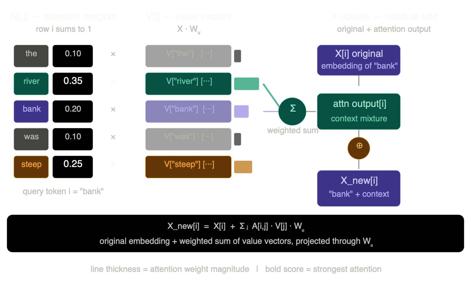
It is remarkable that nearly the entire LLM pipeline will operate on token (resp. embedded vectors) only. Attention is the only part, where relation between objects is established, captured and accounted!
Why multiple heads?
A single attention pass can only learn one type of relationship at a time. The word “bank” might need to attend to “river” for disambiguation while simultaneously attending to “deposit” for grammatical agreement. Two different relationships that cannot be captured by a single weighted sum. Multi-head attention runs several attention operations in parallel, each with its own learned \(Q\)/\(K\)/\(V\) projections. Each head is free to specialize. Empirically, heads tend to learn distinct roles: some track syntactic dependencies (subject to verb), some track co-reference (pronoun to antecedent), some detect repeated patterns. This specialization is not designed, it emerges from training. Another phenomena of end-to-end learning!
The outputs of all heads are concatenated and projected back down to the model dimension, giving one enriched representation per token that integrates multiple relationship types simultaneously.
Got Distracted? - When Attention fails: The attention dilution phenomena
There is a cost to the soft max normalization. Because scores sum to one, attention is fundamentally a zero-sum competition. Every token you attend to strongly reduces attention available for everything else! In a short context window this rarely becomes a problem. In long context sessions, like multi-turn conversation or agentic AI (later more on that), the relevant signal gets shared across hundreds or thousands of tokens, and the weight (influence) on any individual token shrinks accordingly.
This has a concrete practical consequence. Your system prompt, the instructions establishing the model’s role and constraints, appears early in the context, combined with any additional context like Claude skills, MCP definitions and similar artifacts. As the conversation grows, more tokens compete for attention. The influence of that ground truth on later layers progressively dilutes. The model does not forget the system prompt nor any of the fancy stuff you added in the way a human forgets. All the bytes are still there, but the attention weight flowing from those tokens to the current generation step becomes small enough that their semantic influence on the output weakens measurably.
As a rule of thumb you may remember:
Short context:   system prompt captures strong attention weight
Long context:    same tokens, but weight spread thin across the large input
                 → system prompt influence at output layer reduced
This is the mechanical root of why even carefully crafted system prompts sometimes seem to fail in long conversations. This also yields another insight of prompt engineering. Constraints should be placed as close to the next possible being predicted. This essentially translates to the well known pattern of ending the prompt with constraint. Again from a different perspective we arrived by the holy three of prompt design:
[CONTEXT]
In cyber security ...

[QUESTION]
Can you ...

[CONSTRAINTS]
Under any circumstances, to not ...
Connecting back to the MLP
After attention redistributes context across positions, the MLP block processes each token position independently again. To this end, I decided for readability to explain everything on single embedding vectors \(x\) only. Without loss of generality we can easily transfer this understanding to the case of \(X = (x_1, ..., x_N)\), i.e., the state matrix. (Due to independence, we could even calculate all \(N\) MLP Blocks in parallel.)
Attention answers “which tokens matter to this one”. MLP Blocks as discussed next, answers “given this enriched representation, which knowledge is expected to retrieve”. The two operations complement each other: attention is the routing mechanism where the MLP Block is the knowledge store. Getting either wrong propagates errors into the residual stream and compounds through subsequent layers.
A human interpretation of the MLP Blocks
So let us look on the mathematics of MLP first, since I already for shaded the intuition behind them by the last sentences of the previous section.
\[MLP(x) = W_2 · activation(W_1 \cdot x + b_1) + b_2\]where
- W₁ ∈ ℝ^(d × n) — expand to higher dimension
- W₂ ∈ ℝ^(n × d) — project back down
Typically, \(n\) is chosen to be four times the models size \(d\).
So what is the intuition behind this construct. The incoming embedding vector \(x\) is first multiplied by \(W_1\). The matrix multiplication can be understood as selecting specific columns from \(W_1\) depending on the values in \(x\). The columns of \(W_1\) are often associated with keys. In the scope of that interpretation the Multiplication \(W_1 \cdot x\) becomes a key selection. Which keys were selected is decided by \(x\), which is holding all the information about the corresponding token, as well as the contextual enrichment from neighbor tokens due to attention mechanism. So this first inner step will intuitively answer the questions, which “knowledge-keys” contribute to the given, enriched embedding vector \(x\). The activation function serves as a threshold mechanism to only activate the keys with high value (certainty). This threshold mechanism is required since the previously applied attention step introduced influences raised from all other tokens to the one under consideration, even if so small these influences are present! The threshold avoids that these unvoided influences trigger. As a gate-keeper the activation function only allow the relevant keys to pass through.
Next, the outer mapping by multiplication with \(W_2\) will take the vector of keys \(k = activation(W_1 \cdot x + b_1)\) and lookup the corresponding values of \(W_2\) storing the knowledge. So to sum up, \(x\) decides, which knowledge keys \(k\) are activated by utilizing \(W_1\); finally \(W_2\) provides the actual knowledge.
This intuition is captured by the following depiction.
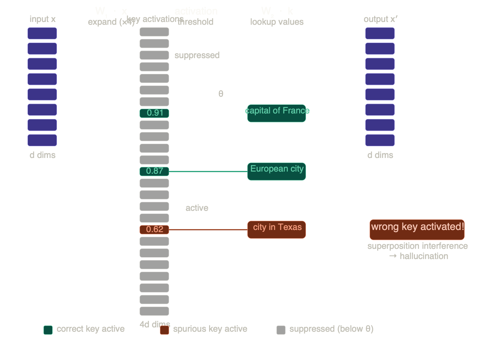
This leaves one final question: How should be chosen \(n\)? The short answer, this is again up to hyperparameter tuning. A too small \(n\) will not be able to capture enough knowledge / information. The same arguments as for the overall model capacity \(d\) holds true here as well. If you think of knowledge as vectors in the models embedding space, you may ask of how much knowledge can be stored in that vector space without interference. I.e., no knowledge is overlapping. The theoretical answer is that this is bound by the dimensionality of the embedding space \(d\). In the embedding space \(d\) we can have up to \(d\) orthogonal vectors, each one composing a “knowledge object”. The dot product of the orthogonal vectors will be null. I.e., there is absolute no interference / relation between them as seen by the model. So since \(d\) is usually small, the dimension expansion to \(n\) allows us essentially to store more knowledge per MLP block. If this is not yet understandable refer back to the discussion of how to choose \(d\).
To even satisfy the modern worlds information capacity demands, another trick is applied named superposition. Instead of taking completely orthogonal vectors, we bias same by small amounts allowing us to increase the knowledge storage a lot. Let me explain this by simple two-dimensional vector space. The unit length vectors \(x = (0,1)\), and \(y = (1,0)\) are orthogonal, i.e., \(dot(x,y) = 0\). However, there exist no more real orthogonal vectors we can add to this set without violating that each vector should be orthogonal to all others. Still, if we accept small “errors” by allowing \(dot(x,y) < 0,123\) we end up with much more vectors, where all satisfies this weakened requirement. The more “semi-orthogonal” vectors allow storing much more information. However, there is a twist. The introduced biases, e.g. \(x=(0.1, 1)\), \(y=(0.9, 0.2)\), etc. will yield that during the multiplication \(W_1 \cdot x + b_1\) keys get activated by accident (refer to above illustration). The small contributions of \(0.1\), \(0.2\) may be sufficient large to trigger the activation function making the MLP Block looking up unrelated knowledge. The unrelated knowledge travels down the layers and end up in something we know as hallucinations.
So to sum up, larger \(n\) correlates with fewer hallucinations for the cost of computational cost impact. Balancing out this hyperparameter is non-trivial.
This brings us to a more broad insight of well-designed prompts. A high information density prompt will yield the containing a lot of non-coherent tokens, will yield heavy activations of key and their corresponding values in the MLP Blocks. These so-called activation of knowledge clusters will yield hallucinations and wrong answers! So a good prompt should always be low-entropy, keep the words and token count of the input in balance (avoid inputs where few words yields many tokens; leave this up to the attackers. They will do anyway.), and keep information density as lows as possible. Anyway, more on good prompt design later, for the moment just remember
Dense prompt:   activates many feature directions simultaneously
                → superposition interference → hallucination risk high

Focused prompt: activates few, specific feature directions
                → features remain approximately orthogonal
                → clean key retrieval → reliable output
To not keep this too abstract, below you find an example of two prompts depicting the concepts learned.
Worse (short but high entropy):
 "Explain how quantum tunneling relates to biological evolution
 and what Keynesian economics says about it"

Better (longer but coherent):
 "In the context of quantum biology specifically,
 explain how quantum tunneling appears in enzyme catalysis,
 focusing on hydrogen transfer reactions"
Notice, the second prompt is longer but activates a coherent feature cluster (quantum mechanics, biology, chemistry), that largely share representational subspace. So it is not about length, it is about token frequency and coherence.
That’s the entire secret about MLP Blocks and the transformer architecture. The remarkable aspect here is, that this matrix never been set by human interaction. The values were initialized randomly like it was the case for the embedding with the sake of the very same argument. During training phase, the values become updated and knowledge get started to be saved in the MLP layer. Another feature of end-to-end learning, and one of the still most interesting topics of research.
Combining it together
So while the input traveling down from layer to layer, at each one, the input sequence dependency on each other is evaluated (attention) and then the state is enriched with knowledge.
It may worse to notice again, that this step is the critical one where the majority of hallucinations occur. We may have a valid tokenization, the positional ordering and embedding is fine, but then the model just selects the wrong knowledge-keys to activate.
Lets “Predict”
Now our input almost traveled until the end of the model. It was tokenized, embedded, enriched by the knowledge stored in the MLP layers, and we arrive at a final state \(X=(x_1, ..., x_N)\) in the embedding vector space. We already have discussed that for the unembedding we now need to apply the inverse operation of embedding only. We discussed how this can be achieved by calculating the dot-products. We also slightly touched how to choose the next token from these dot product values. But for now there is an obvious issue. Since our input was \(N\) token length, we embedded \(N\) tokens, we obtained \(N\) embedding vectors, we updated these \(N\) vectors using attention to introduce relation between them, we fetched the knowledge from the MLP blocks for each of the \(N\) vectors; but the prediction will only be \(1\) token. So how can we reduce from \(N\) to \(1\). The answer is trivial, we just forget about the first \(1, ... (N-1)\) vectors. This is possible since the vector \(x_N\) is already implicitly containing information and knowledge from all the previous tokens due to the many attention and MLP layers. And how to unembed a single vector \(x_i\) should nothing new to us anymore.
Still, there is something new we can learn here. Until now, we just chose the one with the highest score. In this final section let us explore in more detail what this means.
Usually a model will not just provide us the next predicted token. The actual output is a probability distribution generated by a so called softmax layer. So for each possible next token, we know how likely this comes next. However, do not get confused. This probability does not say anything about correctness of that token. It only answers the question of how likely is that token under the constraint of the input tokens provided.
If you think that this probability measure is helpful in judging on the LLM output you are may terribly wrong. Assume that the model says the next token is the given by the highest probability of \(0.51\). Sounds valid, isn’t it? Actually it depends. If there are other tokens like not, having probability of \(0.48\) it becomes questionable if the was the right token to predict next, even if posing the highest probability! To this end modern LLM also account for margins: How big is the difference between the highest probability token and the next k following ones?. Now you can much better spot if the prediction is sound or not. Still remember, this is just how sure the model is that this token follows the previous one. The model does not have any semantic understanding per se. For example top words like the, a and or are seen heavily throughout the training, so the model does have learned semantics of natural language very well and know exactly when of these words have to follow; but contentwise there is no measure of certainty.
So even at this final stage, thinks can go wrong, if using the wrong selection strategy for the next predicted token.
Before moving on to agentic AI let me wrap up the pipeline by one picture.
Wrapping up the Pipeline and putting it all Together
To end this exploration on the LLM, let us shortly depict the entire pipeline architecture. Since an image does say more than thousands words, let me keep this section small by presenting two illustrations only.
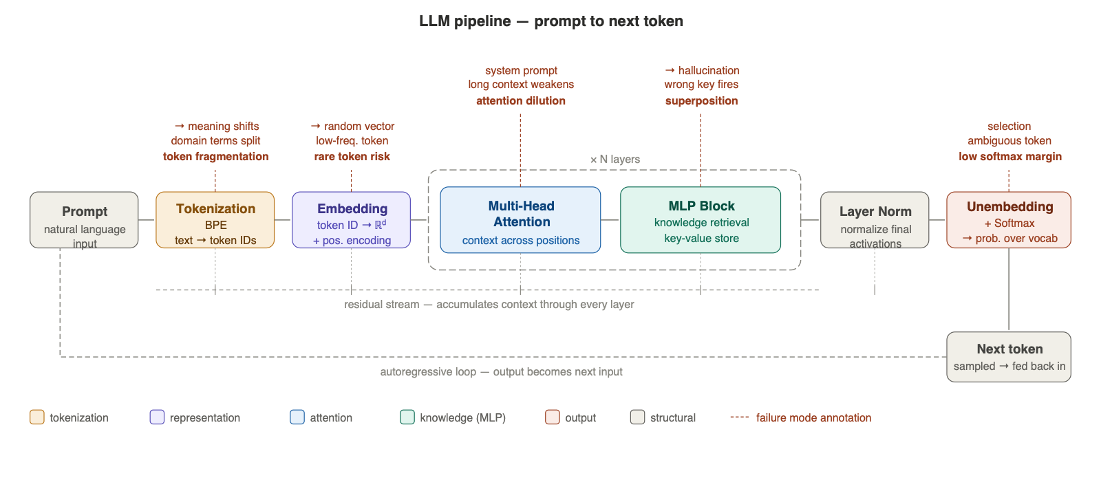
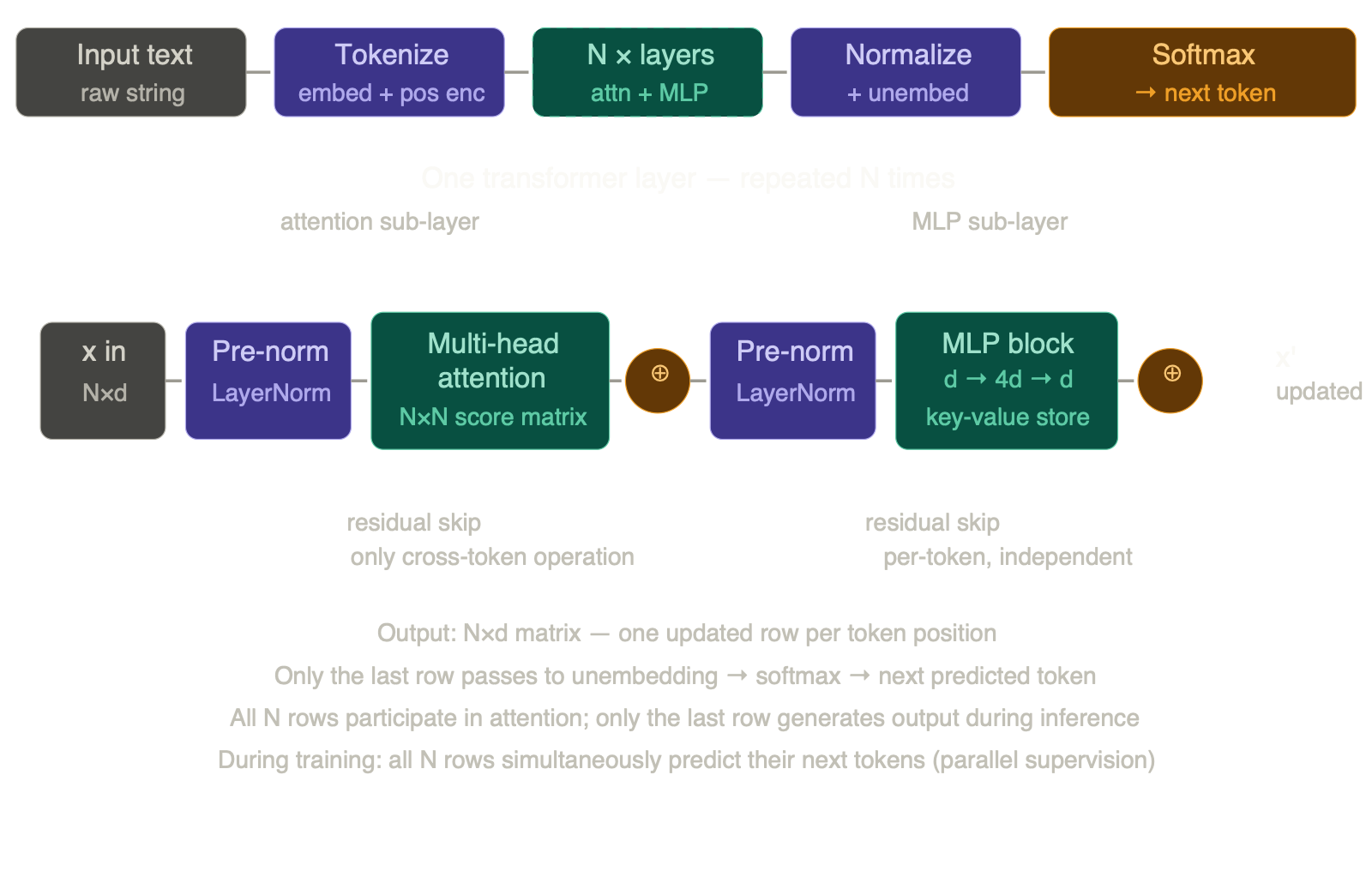
Part II: Agentic AI
In the first part of this long post we discussed the basics of modern LLMs. We have seen how the can misbehave on high entropy input, non-coherent information in the prompt, and high information density input in general. Now let us move on to the Agentic part.
First, we need to define what agentic means. Thanks to commercial marketing everything is understood to be agentic nowadays. Anyway, let us stay with a more robust definition by distinguishing assistive AI against agentic AI
| Agentic AI | Assistive AI | |
|---|---|---|
| Input | Input is consumed from an abstract user goal or the LLM output directly | Basic chat prompt issued by the user |
| Output | Intermediate actions to take. | Answer on the users question. |
| Action | Action inherited by the output. | No actions taken |
So the main difference is, that agentic AI systems are allowed to execute actions based on the LLM results. Another often typically named property of agents is that they operate iteratively. Depending on the amount of iterations we may sometimes call the agent autonomous, if no human interaction is foreseen for a specific amount of iterations (typically until achievement of objectives).
User Goal → LLM → Action → LLM → Action → ... → Output to the user
This chain of actions break us to a major issue with agentic AI. In our basic observations we learned, that LLMs are bad at working on high entropy inputs. However, the output from actions may not always be low entropy. Imaging a malware triage agent is running strings, then decides what to do next. Now the context is infected with high-entropy values. The very some holds true for logs, or errors if tool execution fails. All this contributes into a bad direction may let the LLM fail on its intermediate input. The agent may misbehave by a probability of \(p = 0.05\) on one iteration. Usually agents are thought for the long time autonomous run, executing multiple iterations. The failure rate drastically increases. The question is not if agentic AI will fail. Its more about when it will happen and how we can handle that cases.
Take a look at the following distribution describing the probability \(P(n=k)\) expressing that there is at least one failure in k steps. Notice, that we assume here that each step fails independently with the same probability \(p\). In practice, errors compound. One bad step can corrupt the context, making subsequent steps more likely to fail (increasing \(p\) over iterations). So the formula is actually an optimistic lower bound! Real-world agent failure rates are likely worse than this model predicts. Still, on the other side we assumed a relative large and pessimistic probability of \(p = 0.05\). Anyway, this entire discussion is more about intuition that about values.
\[\begin{align} P(n=1) &= 1 - (1-p) = p \\\\ P(n=2) &= 1 - (1-p)^2 \\\\ P(n=3) &= 1 - (1-p)^3 \\\\ P(n=k) &= 1 - (1-p)^k \\\\ \end{align}\]To state this by numbers, take the following series. For, e.g., \(k=10\) we have already failure probability of \(40\%\). At \(k=50\) it becomes completely unusable. These numbers may sound high, but if you think about your coding assistant and how many iterations it executes before finishing a code.
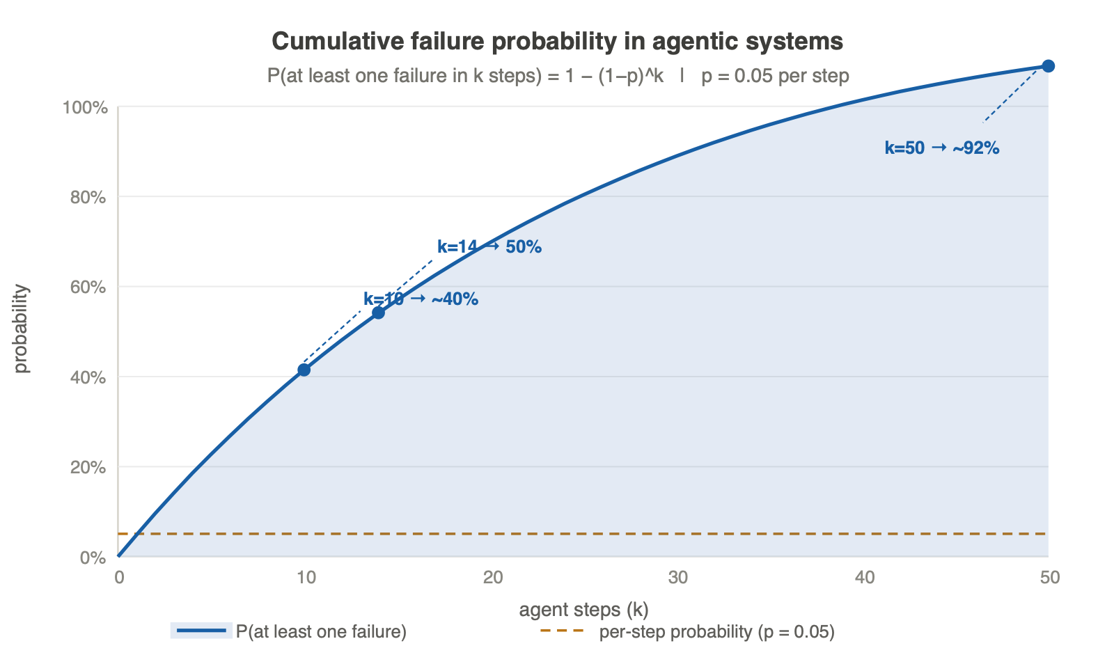
So how can we circumvent this problem? There are actually two ways only
- Decrease the failure probability of LLMs to zero. Just not possible!
- Implement human checkpoints, where a result is verified by a human operator making sure the agent is running as expected
A notable observation is that if the human is assumed to spot the intermediate error and can correct it, the probability chain discussed above resets. This means we do not have to check the agent on every instruction, but from time to time we should keep an eye on it. All this does not yet have discussed cases of adversarial inputs increasing the failure rate drastically if crafted correctly.
So is this all for agents? Just inserting human checkpoints, and we are good to go? Not really, there is another problem concerning the context window size. So with every iteration the initial goal of the user vanishes more and more being not present in the last iterations anymore. A concrete example
→ User requests to fix the unit test
→ AI does a first change; something else breaks
→ AI now says I have to avoid that unit tests from failing
→ Another correction and failure iteration
→ AI now says avoid that unit test failing
→ AI decides to delete the unit tests
→ User sees output "Done no more failing unit tests"
For sure this is a very constructed example but still it should warn us about something. I initially implemented the malware triage agent in the last blog post. While I worked on this I observed something surprisingly. I initially let handle the AI the entire workflow. The agent tried to spawn a docker container, which failed since docker was not installed in my lab. So the agent tried to fix this. All this pulled a lot of information in the context. Still the agent failed on that due to missing privileged access. The LLM was searching how to handle this. In the end it came up with the solution to execute the python scripts, which initially were designed to run inside the docker container, on the host. So the constraint of do not execute anything on the host was simply aged out due to intermediate tool failure and context overflow. In my case nothing happened, but you can imagine the catastrophic situations may occur. While the probability is low, the risk is real. Just because something did not yet happen in your life it does not mean it can’t anymore!
So this sounds all terribly frustrating and sad. I have to agree on it, and was demonstrating extreme cases here. Still this may learn us awareness on how we architect good agents.
Below is a list of key design principle I use when working with AI:
- Entropy control via input filtering. Never feed the LLM with entropy low structured input at any time (“Entropy Firewall”)
- Additionally, you may like to filter the input using the presented heuristics on vocabulary coverage and token frequency
- Deterministic preprocessing pipeline: Any pre-processable task should be conducted out of band. Only tool results should be feed to the LLM.
- Bound the privilege scope of our LLM and any tool it may need to execute (Principle of The Least Privilege)
- Isolated execution environment, whenever possible
- Neutral prompt framing: If your application needs to decide about a topic to not use any keyword in your prompt directing the model into a specific direction. E.g., the malware triage classifier should not contain the word malware in its prompt!
- The agent exactly what you did not want. This will yield negative space disambiguation, disabling the corresponding knowledge cluster
- Request explicit reasoning extraction: Reasoning extraction is the log of a LLM. If anything goes wrong, thus you know at least why!
- Apply human checkpoints to verify the reasoning (not just the result)
If you keep with these principals, you still are not safe from failure but you may minimize it. Still there are fundamental issues not be able to avoid. For the sake of completeness I will try to identify at least some of them I thought of while writing this post:
- The Key activation issue: Certain keywords activate specific knowledge in the LLM yielding a drift from the initial desired task. E.g., assuming you are using Claude Code with custom skills. Now you have a lot of skills on password security, password managers and phishing resistant authentication. You now decide to implement a malware classifier like we have done in the previous post. During runtime of Claude, the skills description will be in the context may yield buzzwords like authentication, passwords and similar in the context as well. Now the agent hits a ransomware. It parses the imports, the strings, and any IoC; but all these IoCs are present in password managers as well. Due to the presence of the keyword. The agent may falsely assume that the sample is a password manager and not a ransomware. A critical false positive. The point with this example is, that even with human inspection you may, would not have observed this during an intermediate checkmark, just because the context window looks benign. We have to accept, that the LLM can see thinks being hidden in front of us. This is what makes them so surprisingly strong and dangerous at the same time.
Thinking in detail about possible failures, we will likely find some more. Still this post is not about complaining AI, it is about making users aware of the risks and to minimize them whenever possible.
Part III: The Divergence Problem
All previous parts just discussed theoretical insights. By this final part I want to bridge to real world AI deployments. Working out something I denoted as the divergence problem. We will see that the specific field (cybersecurity, user desires, market demands) does not always align well with the requirements of safe AI deployments. The arguments are based on theory, still being subjective and momentary. Any change in the AI landscape, which is currently very dynamic, can change everything! This is also the reason I put this section last. So while reading the next sections keep this in mind.
The Divergence in Cybersecurity
A question went viral in the 2025 was, whether AI will replace my (your) job. This superficial question does actually hide a more relevant question, whether AI nature aligns well without domain specific data. The answer to this question is very domain specific. For some fields the honest future will maybe replacement, while others are not replaceable at all. My following argumentation will be just about my field: Cybersecurity
So how well aligns the “Cybersecurity data” with the nature of AI, especially LLMs?
During that post we learned about the three major impacts contributing to bad classification in LLMs, namely the entropy, information density (coherence) and input length in general. For the case of automated and autonomous malware analysis and classification, we already discussed the miss alignment and holistically denoted malware as the natural enemy of LLMs. The reason was exactly that high entropy, and information density. However, cybersecurity is more than just malware analysis, which makes the situation actually worse! In this post we worked out, that LLMs benefit from domain specific training. My major argument here is that Cybersecurity is not just one domain (or at least not a small one) in the sense of AI models. Already the malware example makes something clear. A LLM trying to classify, e.g., a credential stealer, does need to have knowledge in the fields of encryption, networking, an where credentials are stored. Stepping ahead and thinking about automated agentic AI driven log processing in SIEMs the situation becomes even more worse. Log data is high information density by nature; not yet arguing about the amount of log data generated in an enterprise. So the logs to be analyzed by the LLM will by high non-coherent covering networking, file system, registry, and any even non computer science related field activated by accident due to its presence in filenames, URLs or usernames. So feeding log data into a general purpose model we are used to using nowadays will yield activation of many misleading MLP knowledge clusters. Imagine you are a token in the input stream and all the other tokens try to pull on you by their attention. You will literally be ripped. Expecting a helpful result from such a disrupted token may become more a desire than a fact. This holds even true, if you want to expect the model to summarize a text covering multiple domains.
So to sum up, already the input data (logs, malware sample, etc.) does not align well with LLMs. However, there is another issue in cybersecurity. Usually cybersecurity means being confronted with people or groups explicitly trying to break the boundaries. These additional threats add in.
To put the nail on the head, let us end with a “LLMs work best if, … but Cybersecurity demands …” comparison
| What LLMs like | What Cybersecurity provide |
|---|---|
| Input entropy is low | Involves maximum entropy inputs |
| Tasks are bounded in scope | Requires unbounded novel reasoning |
| Context is non-adversarial | Is defined by adversarial context |
| Synthesis can be avoided | The work is fundamentally synthesis |
| Failure is recoverable | The decisions involves irreversible consequences |
The Divergence from Users Perspective
Users not enabled to build AI applications whose code they could not have written on their own, yielding a lot of applications created by developers who were not able to understand their products code. Without understanding the product, you will now be able to judge on whether it is safe or secure to use. Due to the low failing probability and missing visibility of “AI mistakes”, our confidence in the LLMs results increase. The latter also increases the impact due to trust based wider application of vibe coded software. Since risk is defined by the product of probability and impact, even with small failing probability naturally the risk increases. Since social media primes us more and more to use AI on every task, like appointment planning, email summarization, file system structure assistants, etc., and nobody wants to be left behind missing out the AI boom, more and more data is processed by AI. On a single failure or adversarial influence all these confidential data may be impacted. According to my observations the average user presenting her/his AI usage on social media, does violate the least privilege and controlled LLM input principles by design. Additionally, the medial hype does prime society more and more into autonomous AI operations. Users will increasingly request the chatbot or AI agent just for a result skipping the reasoning. However, if reasoning is omitted the output can not be verified anymore. All this may yield, that we lose our capability of critical thinking and questioning. I personally see an increasing trend with more dependence on AI. My final recommendation is that you should work with AI in such a way that you can always continue to work the next day without AI. Enable explicit reasoning extractions, question the models claims and use LLMs as your thinking partner not problem solver! This may be the only way to stop this divergence.
The Divergence between Market demands and safe deployments
On the large scale the divergence problem shows up in current market grows. Nearly every day a new AI feature is released. Everybody is afraid of losing the AI race. The models context size increases above ridiculous sizes. The models trend into general purpose ones, just to sell more. All this does not scale will with the current LLM transformer architecture. Anyway, as long as the market is driven by money and fear of missing out, this divergence between safe AI deployments and the current market developments will remain.
Conclusion
AI and AI agents entered our every day life and will not go away anymore. More and more people will start build amazing new tools, agentic systems and enrich this world by just using natural language. While this development is a big enabler, it also yields safety and security risks. With every 100th well-designed AI application there is may one catastrophically failing. The growing market shares demand the AI developers to provide more and more general purpose models, not trained on domain knowledge, with increasingly capabilities and ridiculous context window sizes. However, after reading this post you will likely observe the divergence with safe AI deployment strategies. These opposite goals do not align well and may yield in personal and/or financial loss at some point. All this said, LLMs became a strong enabler. They allow us to speed up code generation. Automate tasks, we were simply not able to automate some years ago due to there non-deterministic nature. The important aspect separating the short-time winners from the long-term ones will be the understanding in basic AI principles. It is not about understanding every detail, work through every and each proof. No, this will just slow you down. The nowadays art is to develop new AI applications but while doing so keep the intuition and pitfalls in your head at least. If you follow this approach you will likely have an awesome future a head. So far my opinion on agentic AI, LLMs and the current situation in social media.
While theoretical diving deeper into the topic and elaborate on the adversarial part is possible, let us stop here for today. May in an upcoming blog post/series I will write about (indirect) prompt injections, context shifting using the crescendo jailbreak, or knowledge cluster blending attacks. The knowledge gained from this article will help us a lot to understand and build our own attacks, and not just copying working examples. Anyway later more on that.
Que sera, sera!